Density Functional Theory and Defects in Semiconductors
Stefan Ask Erik Elfgren Isak Jonsson
Mars 2000
PROJECT REPORT
Department of Mathematics
A review is given on the Density Functional Theory (DFT) along with its applications
on silicon and carbon, materials important for the semiconductors.
Some related concepts, like exchange-correlation energy are also explained briefly.
The Density Functional Theory is compared to its predecessors as well as
to the Hartree-Fock theory. Furthermore, the characteristics of silicon and carbon
are discussed - the possible structures and symmetries as well as their physical properties.
This study is made as a preparation for making a thorough investigation of silicon
carbide, which is very interesting for extreme environments.
A theoretical section on group theory is also included for the sake of completeness.
Finally, the implementation of
DFT calculations is treated and some practical calculations are presented. For silicon
and carbon structure optimizations are made and the energy levels are calculated.
With DFT, the structure is calculated for the diamond structure. First
as a normal lattice, then with an interstitial or a vacancy.
¯Keywords: Density Functional Theory, Group Theory, Semiconductors,Silicon, Carbon
In todays society semiconducting materials play an extremely important role in making tools and gadgets that are used daily, such as personal computers, mobile telephones and so on. As the use of semiconductors in electronics is totally based on defects in the materials it becomes crucial to understand the behavior of these defects at a microscopic level to make further progress in this area. The defects can be of beneficial as well as destructive character. In the production of semiconding components a lot of defects are introduced in the material. Some of these defects are wanted but there are also a lot of interfering defects. Often, defects are introduced purposely in semiconductors to change e.g. the conduction properties. This process is called doping and the wanted defects are interstitial atoms and vacancies. In contrast, the unwanted defects can also be of different character such as line defects or piling defects.
The most widely used semiconducting material is silicon (Si). Silicon does not always have the best properties for applications, but it is very easy to manufactor. Its ability to reduce defect concentration (by heating the structure to make it relax and then let it cool down) is very efficient. However, in tough environments this very property is also its weakness. In these cases other semicondutors, such as silicon carbide and gallium nitride, might be the only solution. These materials are much more resistant and therefore better suited for most applications. However, they are also very difficult to dope, which makes them very hard to manufacture and therefore they are only used when really needed. Due to their excellent properties one hope to be able to control the defects better in these materials in order to profit more widely from their benefits. For example, electronics could be made to work at higher frequencies, thereby increasing their efficiency, due to the high thermal resistance of these kinds of materials.
The aim of semiconductor physics is to gain control over the defects in the material, thereby controlling its properties. This is desirable to exploit the good effects as well as to negate unwanted defects.
To be able to study defects in semiconducting materials, as in all scientific research areas, a mathematical model is needed. This both to interpret experimental results as well as to predict phenomena not yet discovered. A mathematical model can, after proper verification, also be used to predict properties that are without reach of experimental detectors. The most accurate model for microscopic physics is undoubtly quantum physics. However, for larger systems the exact quantum mechanical treatment is by far too complicated to be solved even with numerical methods, even less then analytically. Different approaches are available to solve this kind of problem. One possibility is to make physical approximations, supported by experimental results. Another is to make a cunning physical model so that experimental data can be dispensed of. Clearly, this is particularly desirable in cases where experimental data are hard to obtain. It might be possible to find another, equivalent but simpler, representation of the system. Such a model is called ab initio (latin for "from the beginning"). This is necessary for having a physically satisfying model and crucial for areas where experiments cannot be performed.
To completely describe the system with quantum mechanics is virtually
impossible, and will certainly remain that way. The exact Schrödinger
equation would contain roughly ![]() terms and about
terms and about ![]() variables for a typical crystal. Hence, approximations are
indispensable. Below is a description of the two main ab initio models.
variables for a typical crystal. Hence, approximations are
indispensable. Below is a description of the two main ab initio models.
The traditionally employed method is the so called
Hartree-Fock model. This model describes the system as a combination
of anti-symmetrical one-electron wave-functions. Thus for a real crystal,
the equations to be solved is still a function of about ![]() variables.
This obliges us to limit the calculations to a very tiny fraction of the crystal
(at most about a hundred atoms) repeated with periodical boundary-conditions
throughout the crystal. Obviously, this affects the result of
defect calculations, as the defects are also repeated. Even with this,
the number of variables is
high, at least in the order of 4N, where N is the number of electron used
to describe the system (normally the valence electrons). In this region, the equation can be
solved iteratively, but in most cases important physical properties are lost.
Hartree-Fock theory is widely used in the chemistry
community but to make this theory accurate enough, perturbation
theory, and such, must be employed which makes larger calculations
practically unfeasable with todays computational systems.
variables.
This obliges us to limit the calculations to a very tiny fraction of the crystal
(at most about a hundred atoms) repeated with periodical boundary-conditions
throughout the crystal. Obviously, this affects the result of
defect calculations, as the defects are also repeated. Even with this,
the number of variables is
high, at least in the order of 4N, where N is the number of electron used
to describe the system (normally the valence electrons). In this region, the equation can be
solved iteratively, but in most cases important physical properties are lost.
Hartree-Fock theory is widely used in the chemistry
community but to make this theory accurate enough, perturbation
theory, and such, must be employed which makes larger calculations
practically unfeasable with todays computational systems.
In the sixties, a new model for multi-particle quantum systems was developed, called Density Functional Theory (DFT). In this model the electron density was proved to be an equivalent representation for the ground-state system. This astounding breakthrough made it possible to completely describe the system with merely the three space-coordinates. In order not to have too many terms in the Schrödinger equation, we still need to limit the system in size. However, the limit is much higher than for Hartree-Fock; we can use about a thousand atoms within reasonable computational power. The DFT also opens up the possibility to make calculations locally in the crystal, so that periodicity is not longer required, thus improving the defect modeling. The original theory, making way for modern DFT, was developed mainly by Walter Kohn, Pierre Hohenberg and Lu J. Sham in the 1960's. The quantum mechanical description with DFT was rewarded with the Nobel Prize in chemistry to Walter Kohn in 1998.
Another crucial tool for making calculations of systems of relevant size is group theory. In the case of semiconductors, group theory treats symmetrical properties of the system and thereby simplifies the problem a lot without any approximations. Crystal structures, like most semiconducting materials, are highly symmetrical and thus, group theory is a very powerful tool in this context. The symmetries can for example be used to find suitable boundary conditions.
Our aim has been to make an initial study preparing for structural calculations of Silicon Carbide. To be able to understand and interpret the behavior of Silicon Carbide, a thorough understanding of the constituents is needed. Hence, we began with calculations for Silicon and Carbon, separately. In these cases, we studied interstitial atoms as well as vacancies and how these defects change the structure and ground-state energies of the materials. These are the kind of defects previously mentioned to be of such importance for doping of semiconductors.
Density Functional Theory (DFT) was applied as the instrument for calculating these structures due to its ability to make accurate calculations in a reasonable amount of time. It would have been possible to employ other methods, as Hartree-Fock, but the calculations would have taken much more time. Hartree-Fock calculations provide more information on the system (like excited states), but we were primarily interested in the ground-state configuration and energy. For theses purposes, DFT is an excellent method.
The calculations were made with a program AIMPRO, Ab initio modeling program, developed for DFT calculations on atomic systems. The program was run in parallel on supercomputers at LTU, UmU and KTH.
To understand this extremely complex problem and its physical description we start, in chapter one, with some relevant notions in quantum physics. From there we proceed to the theoretical description of Density Functional Theory. In chapter two, we continue with an introduction to group theory and its applications in crystalline materials. In chapter three we explain some properties of semiconductors in general and silicon (Si), carbon (C) and silicon carbide (SiC) in particular. Further, in chapter four we present our calculations and results regarding the behavior of vacancies and interstitials in silicon and carbon. Finally, chapter five contains a summary of our work and some conclusions about the different semiconducting materials treated.
We are greatly indebted to our supervisor, Sven Öberg for his untiring interest and support. In particular, his assistance with
the calculations in the final stage of the project has been of great value.
We also express our gratitude to High Performance Computing Center North, (HPC2N)
, and the department of computer added design at LTU for allowing us
to use their computational capacity.
for his untiring interest and support. In particular, his assistance with
the calculations in the final stage of the project has been of great value.
We also express our gratitude to High Performance Computing Center North, (HPC2N)
, and the department of computer added design at LTU for allowing us
to use their computational capacity.
To be able to see more clearly what a huge impact the Density Functional Theory (DFT) has, some quantum mechanics is briefly treated followed by a primitive predecessor to DFT, the Thomas-Fermi model. The chapter culminates in the very method of DFT in section 2.3.
In order to understand the full width of the problem of calculating the structure and properties of a crystal the complete Schrödinger equation will be presented in this section. In the following section, the Born-Oppenheimer approximation is discussed which makes the problem a lot easier, but still far beyond our grasp. The solution is postponed until it can be discussed more though roughly in sections 2.2 and 2.3. Further, the variational principle is stated (rather mathematically), and the definition of electron density in a multiparticle system is given. Finally, some notions (exchange and correlation energy) connected to the most common and reasonable methods for solving the Schrödinger equation are treated in sections 2.1.5 and 2.1.6.
The time independent Schrödinger equation for N spinless electrons with ![]() ions (with
charge
ions (with
charge ![]() ) is
) is
![]()
where ![]() is the total energy of the system and the wave-function
is the total energy of the system and the wave-function
![]()
gives all information there is to know about the system. Here the ![]() denotes the position
and spin, respectively of electron i and
denotes the position
and spin, respectively of electron i and ![]() the position and spin, respectively of atom i.
Effectively, the wave equation depends on
the position and spin, respectively of atom i.
Effectively, the wave equation depends on ![]() variables. For a typical system,
variables. For a typical system,
![]() , Avogadro's number, and
, Avogadro's number, and ![]() giving a total
number of variables in the order of
giving a total
number of variables in the order of ![]() . Obviously, solving a differential equation with that
many variables is impossible.
. Obviously, solving a differential equation with that
many variables is impossible.
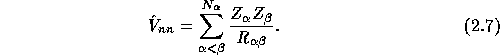
The Hamiltonian for this system has the form
In order not to be encumbered by undesirable units we work in atomic units where
![]() .
This gives the total electronic kinetic energy
.
This gives the total electronic kinetic energy
the total ionic kinetic energy
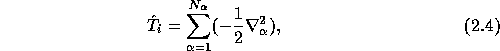
the ion-electron interaction energy
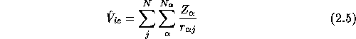
and the electron-electron interaction energy
![]()
and the ion-ion interaction energy
Once again, with normal values of N and ![]() , the Hamiltonian operator achieves
quite frightening proportions. Only the electron-electron interaction energy contains
in the order of
, the Hamiltonian operator achieves
quite frightening proportions. Only the electron-electron interaction energy contains
in the order of ![]() terms. The Schrödinger equation to be solved is
therefore of the form
terms. The Schrödinger equation to be solved is
therefore of the form
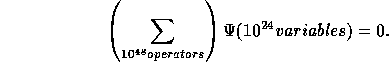
Impossible to solve, indeed!
In the system, the electrons move very fast in comparison with the ions, due to their
mass ( ![]() ). Thus we can approximate that the electrons can
configure themselves as if the ions were fixed. The ions make a
(positive) background, not effecting the states of the electrons except as a
potential. Conversely, the ions don't depend on the fast moving electrons.
This is called the Born-Oppenheimer approximation.
The electrons are (partly) decoupled from the ions which means that the wave function can be written as:
). Thus we can approximate that the electrons can
configure themselves as if the ions were fixed. The ions make a
(positive) background, not effecting the states of the electrons except as a
potential. Conversely, the ions don't depend on the fast moving electrons.
This is called the Born-Oppenheimer approximation.
The electrons are (partly) decoupled from the ions which means that the wave function can be written as:
![]()
where the ![]() and
and ![]() describes, respectively, the ionic and the electronic
part of the wave-function and
describes, respectively, the ionic and the electronic
part of the wave-function and ![]() , and
, and ![]() are the spatial and the spin coordinates, respectively of the ions
and the electrons. As the Born Oppenhemier approximation is fairly closeto the reality it will be used henceforth.
are the spatial and the spin coordinates, respectively of the ions
and the electrons. As the Born Oppenhemier approximation is fairly closeto the reality it will be used henceforth.
The Born-Oppenheimer approximation gives the new Schrödinger equation (for the electrons):
with ![]() and
and ![]() defined as in section 2.1.1.
The energy found, E, depends on the ion-potential, which is a function of
(
defined as in section 2.1.1.
The energy found, E, depends on the ion-potential, which is a function of
( ![]() ). Hence,
the electron energy is also a function of these variables.
When we want to find out the total energy of the system we must, of course, also
include the ionic part. The Born-Oppenheimer approximation is semi-classical
as the electron energy is introduced as a potential energy when solving the ionic
system. In other words, the electron - ion interaction is made classically, though
their structures each for themselves are calculated quantum mechanically.
). Hence,
the electron energy is also a function of these variables.
When we want to find out the total energy of the system we must, of course, also
include the ionic part. The Born-Oppenheimer approximation is semi-classical
as the electron energy is introduced as a potential energy when solving the ionic
system. In other words, the electron - ion interaction is made classically, though
their structures each for themselves are calculated quantum mechanically.
However, even with this approximation the problem of solving the electron wave-function is impossible. We now have only one type of particles, which is a progress indeed, but the number of variables is only decreased marginally and so is the number of terms of the Schrödinger equation. Solving this without further approximation is impossible, but before attempting this, a few more definitions in quantum mechanics is needed.
For a state ![]() , which may or may not satisfy the Schrödinger equation (2.2) (or (2.9)),
the expectation value of the energy operator is
, which may or may not satisfy the Schrödinger equation (2.2) (or (2.9)),
the expectation value of the energy operator is
![]()
The ground-state energy, ![]() is obviously the minimum of
is obviously the minimum of ![]() with respect to
with respect to ![]() :
:
![]()
The variational principle states that the wave-function is stable in its ground state:
This ![]() is the ground-state and thus it satisfies the
Schrödinger equation (2.2) (or (2.9)). N.B. that equation (2.12) can
also be satisfied for local minima (or maxima) of the energy with respect to the wave-function.
Thus, if the condition is satisfied, it is still possible that we've only found a meta-stable
position.
is the ground-state and thus it satisfies the
Schrödinger equation (2.2) (or (2.9)). N.B. that equation (2.12) can
also be satisfied for local minima (or maxima) of the energy with respect to the wave-function.
Thus, if the condition is satisfied, it is still possible that we've only found a meta-stable
position.
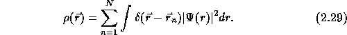
The electron density ![]() is a function of the three space variable
is a function of the three space variable ![]() which is
normalized so that the integral equals the number electrons:
which is
normalized so that the integral equals the number electrons:
![]()
The electron density in itself is given by the solution of the Schrödinger equation (2.9) through
where ![]() are the spatial and the spin coordinates.
The electron density is a key concept in DFT, though it is not considered through the wave function above,
except for theoretical purpose in order to prove the validity of the theory.
The total wave function is never calculated and
the electron density is an independent object which replaces the wave function.
are the spatial and the spin coordinates.
The electron density is a key concept in DFT, though it is not considered through the wave function above,
except for theoretical purpose in order to prove the validity of the theory.
The total wave function is never calculated and
the electron density is an independent object which replaces the wave function.
The exchange energy is the effect of the Pauli-principle which tends to reduce the probability of electrons to occupy the same point in space. If the Schrödinger equation (2.9) would be solved exactly, the exchange energy would be included in the solution. Unfortunately this is not possible and we are forced to solve for each electron separately and then introduce the exchange effect separately. The exchange part wants to make the total wave-function antisymmetric and is thus non-local.
The correlation energy is also stemming from the fact that the Schrödinger equation (2.9)
is not solved exactly. The origin is more intricate than that of the exchange energy
but has to do with the fact that the wave-function doesn't want to be wrinkled
(because of the second derivative in the kinetic energy). Quantum mechanically this can be described
using a linear combination of Slater determinants used in e.g. Hartree-Fock theory, but
the number of determinants needed is huge, often millions, making the method
unrealistic. This is called configuration interaction.
In Density Functional Theory, the correlation energy can be naturally included without
using millions of Slater determinants like in Hartree-Fock Theory.
The heat capacity of metals can be accounted for with the correlation energy. Hence,
DFT is generally much better for these kinds of calculations than is Hatree-Fock.
In general the correlation energies are an order of magnitude or more, lesser than the exchange energies
Let us now turn to the problem of solving the Schrödinger equation of section 2.1.1, with billions of billions of terms and variables. As we have mentioned earlier, we must make an ansatz for the solution, limiting the possibilities. Even though the results of Thomas-Fermi model in themselves aren't remarkable, it is the foundation of DFT, and as such deserves some attention.
The idea in the Thomas-Fermi model is to replace the complicated N-electron wave function
![]() with the charge density
with the charge density ![]() thus reducing the degrees of freedom from 4N (three spatial- and one spin-coordinate) to
only three spatial coordinates. The transition from the quantum mechanical
thus reducing the degrees of freedom from 4N (three spatial- and one spin-coordinate) to
only three spatial coordinates. The transition from the quantum mechanical ![]() to the
global variable
to the
global variable ![]() can be achieved by using several different approaches.
The one presented, rather briefly, in this section will use statistical considerations.
can be achieved by using several different approaches.
The one presented, rather briefly, in this section will use statistical considerations.
The energy of a particle in a three-dimensional well is
![]()
This gives ![]() , the density of states, as:
, the density of states, as:
![]()
with R defined implicitly above. The electrons are fermions and in order to treat them statistically, we have to employ Fermi-Dirac statistics. The Fermi-Dirac distribution function is
![]()
where ![]() is the chemical potential,
is the chemical potential, ![]() is the temperature,
is the temperature, ![]() is the Boltzmann constant,
is the Boltzmann constant,
![]() is the step (also called Heaviside) function and
is the step (also called Heaviside) function and ![]() is the Fermi-energy.
Thus, in the zero temperature limit we have
is the Fermi-energy.
Thus, in the zero temperature limit we have
![]()
where ![]() is a proportionality factor and the 2 comes from the fact
that we have two electrons (with different spin) in each point. This means that the Thomas-Fermi
kinetic energy is expressed in terms of the electron density as
is a proportionality factor and the 2 comes from the fact
that we have two electrons (with different spin) in each point. This means that the Thomas-Fermi
kinetic energy is expressed in terms of the electron density as
![]()
where ![]() has been eliminated by the use of
has been eliminated by the use of ![]() and
and ![]() .
.
Finally, the energy-functional that is to be minimized is:
![]()
This gives the Euler-Lagrange equation (cf. appendix A, section A.3):
where
is the (classical) electrostatical potential.
The difference between the Thomas-Fermi and the Thomas-Fermi-Dirac (TFD) model is that the TFD model includes the Hartree-Fock exchange-energy functional:
![]()
where ![]() is defined as the exchange energy from Hartree-Fock theory, a (normally non-local)
interaction term between different parts of the electron density:
is defined as the exchange energy from Hartree-Fock theory, a (normally non-local)
interaction term between different parts of the electron density:
where ![]() and
and ![]() are the other variables. We note that
are the other variables. We note that
![]()
is the normal electron density (cf. equation (2.14) with ![]() being included in the integral).
If we approximate that non-local effects can be ignored
the Dirac exchange energy can be expressed in terms of the electron density directly:
being included in the integral).
If we approximate that non-local effects can be ignored
the Dirac exchange energy can be expressed in terms of the electron density directly:
where ![]() .
The energy functional thus becomes:
.
The energy functional thus becomes:
![]()
with ![]() defined as in (2.20).
defined as in (2.20).
![]()
where ![]() may, or may not be the Coulomb potential.
Hohenberg and Kohn (1964) and Kohn and Sham (1965) showed that for every potential
may, or may not be the Coulomb potential.
Hohenberg and Kohn (1964) and Kohn and Sham (1965) showed that for every potential ![]() ,
there is exactly one corresponding electron density:
,
there is exactly one corresponding electron density:
The electron density gives the number of electrons and determines, through the
![]() in the Hamiltonian, the ground state of the wave-function.
In other words there is a one-to-one correspondence between the electron density and the
ground state wave-function. However, the correspondence is not onto, i.e. not all electron
densities can be represented by a potential.
in the Hamiltonian, the ground state of the wave-function.
In other words there is a one-to-one correspondence between the electron density and the
ground state wave-function. However, the correspondence is not onto, i.e. not all electron
densities can be represented by a potential.
![]()
This is the same as saying that the variational principle applies, which is crucial for finding a reliable solution to the problem with a minimization procedure.
:
![]()
so that when an electron density is found only these criteria have to be verified, not that the electron density can be represented by a potential. For the interested reader, the article by Hohenberg and Kohn (1964) [3] is recommended.
To solve the functional we apply our physical boundary conditions for neutral atoms,
![]()
and the Poisson equation to (2.21).
Neither the Thomas-Fermi, nor the Thomas-Fermi-Dirac functionals give any remarkable
results. One of the problems with the models is that they give densities that go towards
infinity as ![]() , i.e. in the vicinity of atomic nuclei.
This can be remedied by the use of higher order
correction terms of gradients of
, i.e. in the vicinity of atomic nuclei.
This can be remedied by the use of higher order
correction terms of gradients of ![]() or by requiring that the electron densities
should have reasonable form. Another problem is that they don't give the proper atomic shell structure.
This is because we have assumed that the kinetic energy only is dependent on
the electron density and not the gradient of it, as might be expected from
the Schrödinger equation. Hence, the rapidly changing
electron density that forms the shell structure cannot be well represented.
or by requiring that the electron densities
should have reasonable form. Another problem is that they don't give the proper atomic shell structure.
This is because we have assumed that the kinetic energy only is dependent on
the electron density and not the gradient of it, as might be expected from
the Schrödinger equation. Hence, the rapidly changing
electron density that forms the shell structure cannot be well represented.
As stated in the Hohenberg-Kohn Theorem, the Schrödinger equation (2.9) for
the ground state energy can be formulated in terms of the three-variable ![]() as:
as:
![]()
with the constraint that
![]()
When this energy is minimized, the electron density satisfies the Euler-Lagrange equation (cf. appendix A, section A.3):
![]()
with ![]() determined by the constraint
determined by the constraint ![]() .
.
The idea of Kohn and Sham was to collect the terms that were non-local together, then to solve each electron individually, with an effective potential formed by the non-local terms. The effective potential is recalculated, and then the electron density is recalculated which in turn give another effective potential. The process is repeated until the energy has stabilized on a minimum. The number of variables and equations are enormously decreased with respect to our original Schrödinger equation (2.9), but definitely higher than the naïve Thomas-Fermi model. In the DFT we still have as many equations to solve as the number of electrons modeled, hence, to model the entire crystal is unthinkable. Normally, we only consider a small part of it, considered to be representative, thus making one more approximation. The scheme of solution goes as follows:
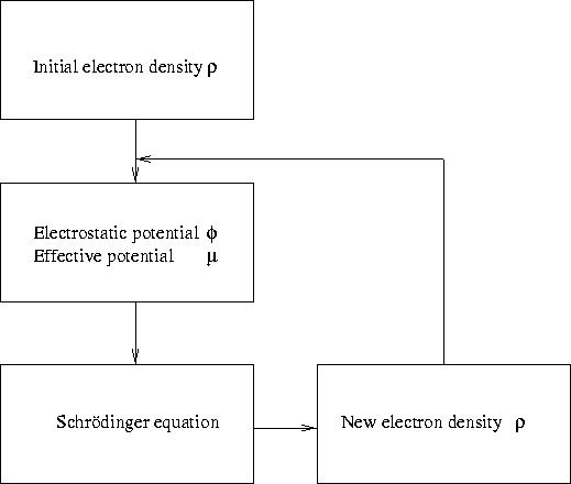
Figure 2.1: Schematic view on the procedure of Kohn-Sham
The energy of a homogeneous electron gas is given by:
![]()
where ![]() is the electrostatic
potential:
is the electrostatic
potential:
![]()
and ![]() is the non-local part of the Schrödinger equation. We separate this functional
in two different parts:
is the non-local part of the Schrödinger equation. We separate this functional
in two different parts:
![]()
where the ![]() is the kinetic energy of a system of non-interacting
electrons and the
is the kinetic energy of a system of non-interacting
electrons and the ![]() is the exchange and the correlation effects (cf. section 2.1.5).
is the exchange and the correlation effects (cf. section 2.1.5).
The one-particle Schrödinger equation that is solved is:
![]()
where ![]() is the effective potential representing the non-local energy
is the effective potential representing the non-local energy ![]() . This
potential is given by
. This
potential is given by
![]()
The result of these equations is used to calculate the new electron density as:
With this ![]() a new
a new ![]() can be calculated and the one-particle Schrödinger equation
can be solved again. This is repeated until convergence.
can be calculated and the one-particle Schrödinger equation
can be solved again. This is repeated until convergence.
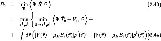
In the presence of a magnetic field our scalar potential ![]() is no longer enough.
Nor is the electron density enough to completely determine the ground state.
As the magnetic field creates a spin-dependent energy, it is natural that the
electron density must be replaced by spin-up and spin-down densities
is no longer enough.
Nor is the electron density enough to completely determine the ground state.
As the magnetic field creates a spin-dependent energy, it is natural that the
electron density must be replaced by spin-up and spin-down densities ![]() ,
, ![]() .
.
The Hamiltonian of the system can be written:
![]()
where ![]() ,
, ![]() and
and ![]() has been defined earlier and
the magnetic energy stemming from the magnetic field
has been defined earlier and
the magnetic energy stemming from the magnetic field ![]() is
is
![]()
where ![]() is the Bohr-magneton and
is the Bohr-magneton and ![]() is the spin for electron i.
The ground-state energy is then given by
{2pt
is the spin for electron i.
The ground-state energy is then given by
{2pt
Let ![]() represent the spin up and the spin-down states respectively
and let
represent the spin up and the spin-down states respectively
and let ![]() or
or ![]() for
for ![]() the number of
electrons in spinstate down and analogously for
the number of
electrons in spinstate down and analogously for ![]() .
If we assume that the magnetic field is pointing in the z-direction,
.
If we assume that the magnetic field is pointing in the z-direction, ![]() the Kohn-Sham equations for the spin density functional theory are:
the Kohn-Sham equations for the spin density functional theory are:
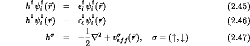
![]()
First, it is only with the supposition that the description of the ![]() is exact that we
get the result of ordinary DFT when
is exact that we
get the result of ordinary DFT when ![]() in spin DFT. However, this is not the case,
and the
in spin DFT. However, this is not the case,
and the ![]() is generally a much better description of the reality
than the ordinary
is generally a much better description of the reality
than the ordinary ![]() is. The latter energy is not well adapted to
unpaired electrons, such as we have for in open-shell molecules. For these cases, the spn-DT is much better to describe the structure.
is. The latter energy is not well adapted to
unpaired electrons, such as we have for in open-shell molecules. For these cases, the spn-DT is much better to describe the structure.
Second, different spins can have different densities, which means that the spin-DFT can include spontaneous magnetization. Hence, the spin-DFT can also be used on materials which have a rather strong magnetic coupling inside. Electronic spin susceptibility can be determined and also spin-orbit coupling and some relativistic effects.
In the Local Density Approximation (LDA) the exchange and the correlation part of the energy
are considered to be local energies, i.e. they are considered to be operating as an effective potential. This means
that the electron wave functions are decoupled and that each electron can be solved separately.
In the LDA-approximation, the exchange-correlation energy is written as
![]()
This is valid only for a slowly varying density and the errors will be of the order of ![]() according to Kohn and Sham 1965 [4].
according to Kohn and Sham 1965 [4].
If we approximate that the correlation energy is varying slowly, thus that it is rather local, we can write the exchange-correlation energy as
where ![]() is the electron density and
is the electron density and ![]() is the correlation energy (cf. section 2.3.5).
is the correlation energy (cf. section 2.3.5).
Without any further approximation we can apply the Hartree-Fock exchange energy ![]() :
:
![]()
where ![]() is defined in equation (2.24)
This gives new Kohn-Sham equations to solve that are much more complicated due to the non-locality.
For the explicit formulas, see Kohn and Sham (1965) [4].
is defined in equation (2.24)
This gives new Kohn-Sham equations to solve that are much more complicated due to the non-locality.
For the explicit formulas, see Kohn and Sham (1965) [4].
If the exchange energy (cf. 2.1.5) also is assumed to be an effective potential (and thus local) we can write
![]()
(cf. section 2.3.3) This means that the Pauli-principle (which governs the exchange energy) will in fact make the electron work "on itself". This is not very physical but the effect is not very large and the results are still respectable. Here, the result from the equation (2.26) can be inserted which gives
![]()
but other possibilities are also available.
There is also a Local Spin Density Approximation (LSDA) for the spin-DFT (cf. previous two sections) which gives the exchange energy functional:
![]()
where ![]() . For further details on this and other
approximations, refer to Parr and Yang (1989) [2].
. For further details on this and other
approximations, refer to Parr and Yang (1989) [2].
In the DFT the correlation energy is rather well accounted for but only approximately. It is not determined universally but a proposition for the high density limit is
![]()
where A and C are constants, see Parr and Yang (1989) [2].
Hartree-Fock accounts for the exchange energy, but not at all for the correlation energy. It is possible to remedy this by e.g. Moller Plesset (or many-body) perturbation theory second-order correction to the Hartree-Fock energy (MP2). However, in order to achieve the same standard on the total energy as in DFT this takes about ten times as long time.
The only disadvantage of the DFT theory is that it only calculates the ground state, not any excited states. This means that it is hard to calculate bandgaps, which in turn makes the DFT theory bad at determining e.g. refraction indices. The Hartree-Fock theory calculates the wave function, instead of just the ground state electron density and it can thus be used to obtain these kinds of informations. There are variants of the Kohn and Sham model where this is also included, but they are not yet fully satisfactory.
The great advantage with DFT is that it is simple and can be made to be an almost complete description, with an energy and an electron density converging to the values of the physical material. This is not acquired in Hartree-Fock theory. For ground-state configurations, the results from DFT are exact and quick. The DFT also allows that a small piece of the crystal is chosen that can be considered as the whole structure, as well as periodic boundary conditions, as in Hartree-Fock. This gives a greater freedom and makes good results easier to obtain.
As in most fields in physics group theory becomes a important
tool to describe the physics in a efficient way. In this case, with
solid state physics, groups of symmetry operations determined
of the crystalline structure are used to simplify the calculations.
We will start with an introduction to group theory, and then show how this
is implemented in solid state physics. In the end of this chapter we
will give a example considering H ![]() O where group theory will be
applied to examine the water molecules properties.
O where group theory will be
applied to examine the water molecules properties.
A symmetry operation is a operation which leaves the object unchanged after operating on it. An example on a symmetry operation is rotation of a spherical object.
A group is defined as a set of elements A, B, C, ![]() that satisfy
the following requirements:
that satisfy
the following requirements:
1. There exists a multiplication operator and the product ofIf a group contain a number, h, of elements then h is said to be the order of the group.any two elements is in the set; i.e., the set is closed under
group multiplication.
2. The associative law holds; A(BC) = (AB)C.
3. There is a unit element E such that EA = AE = A.
4. There is in the group an inverse A
to each element
A such that AA
There are several concepts in group theory that are important for further comprehension of the subject. This section will give a brief explanation of the most important ones that will be used later in the applications of group theory, such as representation of symmetry groups etc.
Isomorphism describes a algebraic relation between groups.
Two groups, ![]() and
and ![]() , are said to be isomorphic if there elements have a
one-to-one correspondence, G
, are said to be isomorphic if there elements have a
one-to-one correspondence, G ![]()
![]() H
H ![]() , which implies
that G
, which implies
that G ![]() G
G ![]() = G
= G ![]()
![]() H
H ![]() H
H ![]() = H
= H ![]() .
If two groups do not have this one-to-one correspondence between
there elements they are said to be homomorphic.
.
If two groups do not have this one-to-one correspondence between
there elements they are said to be homomorphic.
A subgroup is, as indicated by the name, a number of elements, g,
that belongs to a group, ![]() , which satisfy the definition of a group
themselves. This means that a product of any two elements in the
selected subset, that forms the subgroup, must also belong to the
subset, i.e. g
, which satisfy the definition of a group
themselves. This means that a product of any two elements in the
selected subset, that forms the subgroup, must also belong to the
subset, i.e. g ![]() g
g ![]()
![]() g.
g.
Suppose there exists two subgroups, ![]() and
and ![]() , to a
group,
, to a
group, ![]() , that commute, i.e. G
, that commute, i.e. G ![]() H
H ![]() = H
= H ![]() G
G ![]() . Then if
all the elements in
. Then if
all the elements in ![]() can be uniquely described by a product,
G
can be uniquely described by a product,
G ![]() H
H ![]() , then
, then ![]() is said to be a direct product group of
is said to be a direct product group of ![]() and
and ![]() ,
, ![]() =
= ![]() . This implies
that the only element that is common to both
. This implies
that the only element that is common to both ![]() and
and ![]() is
the identity, which is an operator that leaves what it is acting on
unchanged.
is
the identity, which is an operator that leaves what it is acting on
unchanged.
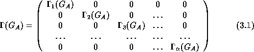
A Class, ![]() , is a definition of similar group elements which are related
through there conjugate elements. A group element, G
, is a definition of similar group elements which are related
through there conjugate elements. A group element, G ![]() , is said to be
conjugate to an element, G
, is said to be
conjugate to an element, G ![]() , if there is an element, G
, if there is an element, G ![]() , in the group
such that G
, in the group
such that G ![]() = G
= G ![]() G
G ![]() G
G ![]() . This implies that if G
. This implies that if G ![]() and G
and G ![]() are both conjugate to G
are both conjugate to G ![]() then they are also conjugates to
each other, i.e.
G
then they are also conjugates to
each other, i.e.
G ![]() = G
= G ![]() G
G ![]() G
G ![]() and G
and G ![]() = G
= G ![]() G
G ![]() G
G ![]()
![]()
G ![]() = G
= G ![]() G
G ![]() G
G ![]() = G
= G ![]() G
G ![]() G
G ![]() G
G ![]() G
G ![]() =
(G
=
(G ![]() G
G ![]() )G
)G ![]() (G
(G ![]() G
G ![]() )
) ![]()
This is the definition of a class, where all the elements are
conjugate to each other. In the same manner it can be derived
that no element can belong to more than one class, because this
imply that those two classes are the same class.
In abelian groups all the elements are there own classes, because
otherwise would the commutation relation give that G ![]() = G
= G ![]() .
.
A representation of a group defines the operators to the different
group elements. Suppose there is a set of linear operators,
![]() (G
(G ![]() ), in a vector space L, which correspond to the elements
G
), in a vector space L, which correspond to the elements
G ![]() of a group
of a group ![]() in the sense that
in the sense that
![]() (G
(G ![]() )
) ![]() (G
(G ![]() ) =
) = ![]() (G
(G ![]() G
G ![]() ),
),
![]() (E) = 1
(E) = 1
then this set of operators is said to form a representation of the
group ![]() in the vector space L. L is called the representation
space of
in the vector space L. L is called the representation
space of ![]() .
.
Abstract algebra is a very general theory, but in practise it is very
common to represent the group elements with square matrices and chose
matrix multiplication to be the group mulitplicantion operator. These
matrices are written ![]() (G
(G ![]() ) and are associated with each group
element G
) and are associated with each group
element G ![]() .
.
A matrix, ![]() (G
(G ![]() ), is reducible if there exists a basis that
makes the matrix more block diagonalized. If this new basis also is
reducible one can proceed and find a basis where
), is reducible if there exists a basis that
makes the matrix more block diagonalized. If this new basis also is
reducible one can proceed and find a basis where ![]() (G
(G ![]() ) can
not be more block diagonalized.
) can
not be more block diagonalized.
This representation, formed by ![]() (G
(G ![]() ),
),
![]() (G
(G ![]() ),
), ![]() ,
, ![]() (G
(G ![]() ), is called
a irreducible representation of the group element G
), is called
a irreducible representation of the group element G ![]() and the set of
, the irreducible representations, for all the group elements then
forms a irreducible representation for the group
and the set of
, the irreducible representations, for all the group elements then
forms a irreducible representation for the group ![]() .
.
When the symmetry operations represented by matrices are invariant under bas transformation it is preferable to also characterize the representations in such a invariant way. This is made through the trace of the matrices, since these are invariant,
![]()
and ![]() is called the character of the
is called the character of the ![]() th
representation. On the basis of the definition of a character it can
be shown that the number of irreducible representations are equal to
the number of classes in the group. It is very common, when matrix
representation is used, that one shows the characters of the
representations in a, so called, character table. In a character table
the columns are labeled by the various classes and the rows by the
irreducible representations, table 3.1.
th
representation. On the basis of the definition of a character it can
be shown that the number of irreducible representations are equal to
the number of classes in the group. It is very common, when matrix
representation is used, that one shows the characters of the
representations in a, so called, character table. In a character table
the columns are labeled by the various classes and the rows by the
irreducible representations, table 3.1.
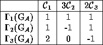
Table 3.1: Example of a character table
In this section we will take a look at the symmetric groups of crystalline solids. A crystalline solid is a regular array of identical unit cells such that the crystal is invariant under lattice translations by
where ![]() ,
, ![]() and
and ![]() are integers and a
are integers and a ![]() , a
, a ![]() and a
and a ![]() are the primitive translation vectors from one lattice
point to an other. But this is not the only operation under which the
crystal is invariant. The complete set of covering operations with one
point (the origin) held fix is called the space group of the
crystal. The group of operations which is obtained by setting all the
translations in the space group to zero, is called the point
group of the crystal. There exist 230 different space groups, and for
crystals there exists 32 point groups.
are the primitive translation vectors from one lattice
point to an other. But this is not the only operation under which the
crystal is invariant. The complete set of covering operations with one
point (the origin) held fix is called the space group of the
crystal. The group of operations which is obtained by setting all the
translations in the space group to zero, is called the point
group of the crystal. There exist 230 different space groups, and for
crystals there exists 32 point groups.
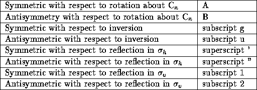
Symmetry operations is normally noted with the Schoenflies
notation, the list below shows the notation of some standard
operations.
E = the identity
C ![]() =rotation trough 2
=rotation trough 2 ![]() /n.
/n.
![]() = reflection in a plane.
= reflection in a plane.
![]() =reflection in the ``horizontal'' plane, i.e the plane
trough the origin perpendicular to the axis of highest rotation
symmetry
=reflection in the ``horizontal'' plane, i.e the plane
trough the origin perpendicular to the axis of highest rotation
symmetry
![]() =reflection in a ``vertical'' plane, i.e one passing trough
the axis with highest symmetry.
=reflection in a ``vertical'' plane, i.e one passing trough
the axis with highest symmetry.
![]() =reflection in a ``diagonal'' plane, i.e one containing the
symmetry axis and bisecting the angle between the twofold axes
perpendicular to the symmetry axis. This is just a special kind of
=reflection in a ``diagonal'' plane, i.e one containing the
symmetry axis and bisecting the angle between the twofold axes
perpendicular to the symmetry axis. This is just a special kind of
![]() .
.
S ![]() =improper rotation through 2
=improper rotation through 2 ![]() /n.
/n.
i=inversion.
This basic symmetry operations can be combined to build up different
groups of symmetry, for example the groups C ![]() contains a
contains a
![]() reflection plane in addition to the C
reflection plane in addition to the C ![]() axis.
axis.
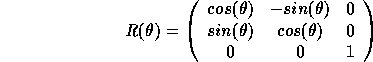
As we mentioned earlier there exists only 32 different point groups in crystalline solids, this is due to restrictions on possible angels of rotation. We can write a rotation as
![]()
We write an three-dimensional matrix for the rotation operation R which carries n into m
If we consider the case when ![]() =
= ![]() =0 and
=0 and ![]() =1, then
m
=1, then
m ![]() =R
=R ![]() i.e R
i.e R ![]() is an integer. Similarly by putting
is an integer. Similarly by putting
![]() =
= ![]() =0 and
=0 and ![]() =1, etc., we can show that R
=1, etc., we can show that R ![]() and
R
and
R ![]() are also integers. Consequently the trace of R must also be
an integer. If we make a similar transformation to a Cartesian set
of basis vectors the trace remains invariant and must therefor still
be an integer. In the Cartesian basis a rotation of a vector trough an
angel
are also integers. Consequently the trace of R must also be
an integer. If we make a similar transformation to a Cartesian set
of basis vectors the trace remains invariant and must therefor still
be an integer. In the Cartesian basis a rotation of a vector trough an
angel ![]() has the trace 1+2cos
has the trace 1+2cos ![]() , because the trace have to be
an integer the only allowed values on
, because the trace have to be
an integer the only allowed values on ![]() are 0
are 0 ![]() , 60
, 60 ![]() ,
90
,
90 ![]() , 120
, 120 ![]() and 180
and 180 ![]() , and hence five-fold axes and
axes of order greater than six are excluded. Similarly for an improper
rotation S(
, and hence five-fold axes and
axes of order greater than six are excluded. Similarly for an improper
rotation S( ![]() ) the trace is 2cos
) the trace is 2cos ![]() -1 and must also be an
integer, so the angel
-1 and must also be an
integer, so the angel ![]() takes the same set of values.
takes the same set of values.
The lattice in eq.3.3 has inversion symmetry, so if it contains an n-fold axis with n>2 it will also have n vertical mirror planes. These conditions, when put together, can be shown to limit the possible number of point groups to 32.
The point groups can be divided in two general categories, the simple rotation groups and the groups of higher symmetry. The simple rotation groups are characterized by a symmetry axis with higher symmetry than the other axes. The groups of higher symmetry have no unique axis of highest symmetry, but more than one n-fold axis, where n>2.
The simple rotation groups is easily visualized bystereographic
projection. Imagine a sphere centered on the origin and mark on its
surface a arbitrary point and all positions to which this point would
move under the group rotations. This can be presented in two-dimensions
by projecting the resulting points on to a plane.
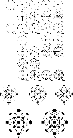
Figure 3.1: Crystallographic point groups.
There are 27 different point groups of the simple rotation type, the stereo-graphic projection of these groups are shown in figure 3.1, together with the five groups of higher symmetry. The points are mapped on to the plane in the following manner, every point i the ``north `` hemisphere is projected onto the equatorial plane by straight line projection trough the ``south'' pole and marked by a cross, and all the points on the ``south'' hemisphere is projected via the ``north'' pole and marked with a circle.
The point groups of simple rotation are
C ![]() : These are the point groups in which the only symmetry consists
of a single n-fold axis of symmetry, the only cases in
crystalline solids are C
: These are the point groups in which the only symmetry consists
of a single n-fold axis of symmetry, the only cases in
crystalline solids are C ![]() , C
, C ![]() ,C
,C ![]() , C
, C ![]() , and C
, and C ![]() .
.
C ![]() : These groups contains a
: These groups contains a ![]() reflection plane in
addition to the C
reflection plane in
addition to the C ![]() axis, this implies the existence of n
reflection planes,
separated by an angle
axis, this implies the existence of n
reflection planes,
separated by an angle ![]() /n around the C
/n around the C ![]() .
.
C ![]() : These groups contain a
: These groups contain a ![]() reflection as well as
the C
reflection as well as
the C ![]() axis.
axis.
S ![]() : These groups contains an n-fold axis for improper rotation
if n is odd, these groups are identical with C
: These groups contains an n-fold axis for improper rotation
if n is odd, these groups are identical with C ![]() and hence they are not
considered. If n is even, they form distinct groups, each of which
includes C as a subgroup. The cases occurring in
crystals are thus S
and hence they are not
considered. If n is even, they form distinct groups, each of which
includes C as a subgroup. The cases occurring in
crystals are thus S ![]() , S
, S ![]() and S
and S ![]() .
.
D ![]() : These groups have n twofold axis perpendicular to the
principal C
: These groups have n twofold axis perpendicular to the
principal C ![]() axis. In D
axis. In D ![]() , therefore, there are three mutually
perpendicular twofold axes.
, therefore, there are three mutually
perpendicular twofold axes.
D ![]() : These groups contains the element of D
: These groups contains the element of D ![]() together with the
diagonal reflection plane
together with the
diagonal reflection plane ![]() bisecting the angels between
the twofold axes perpendicular to the principal rotation axis.
bisecting the angels between
the twofold axes perpendicular to the principal rotation axis.
D ![]() : These groups contain the elements of D
: These groups contain the elements of D ![]() , plus the
horizontal reflection plane
, plus the
horizontal reflection plane ![]() . Hence, D
. Hence, D ![]() , has twice as many
elements as D
, has twice as many
elements as D ![]() .
.
The groups of higher symmetry have, as mentioned earlier, have no
unique axis of highest symmetry but they have more than one axis with
at least threefold symmetry. The five groups in this category are T,
T ![]() , T
, T ![]() , O and O
, O and O ![]() , they only exists in cubic crystals, in
which the fundamental translational vectors are mutually perpendicular
and of equal length. Therefore it will be convenient to consider all
this groups in conjunction with a unit cube.
, they only exists in cubic crystals, in
which the fundamental translational vectors are mutually perpendicular
and of equal length. Therefore it will be convenient to consider all
this groups in conjunction with a unit cube.
T: This group consists of the 12 proper rotations which take a
regular tetrahedron into itself. These operations can be visualized if
we consider the tetrahedron in figure 3.2 which is inscribed in a
cube. The X, Y and Z axes are normal to the cubes faces, and the
origin is in the center of the cube The covering operations of the
tetrahedron are then seen to be: E, C ![]() around each axis and
eight C
around each axis and
eight C ![]() 's about the body diagonals of the cube.
's about the body diagonals of the cube.
T ![]() : The full tetrahedral group T
: The full tetrahedral group T ![]() contains all the
covering operations of a regular tetrahedron, including reflections.
contains all the
covering operations of a regular tetrahedron, including reflections.
T ![]() : This group is obtained by adding the inversion to the group
T. Note that inversion is not a symmetry operation of the
tetrahedron, and are therefore not contained in T
: This group is obtained by adding the inversion to the group
T. Note that inversion is not a symmetry operation of the
tetrahedron, and are therefore not contained in T ![]() . T
. T ![]() is a direct
product group formed by T and S
is a direct
product group formed by T and S ![]() .
.
O: This is the group of proper rotations which take a octahedron,
or cube, into itself.
O ![]() : This is the largest of all the point groups with 48
elements. It is the full symmetry group of a cube or octahedron,
including improper rotations and reflections.
: This is the largest of all the point groups with 48
elements. It is the full symmetry group of a cube or octahedron,
including improper rotations and reflections.
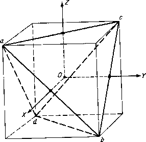
Figure 3.2: Tetrahedron inscribed in a cube.
The crystallographic point groups are a very handy tool to use in calculations. The different symmetries of a crystalline solid can be used to simplify a problem, so that it can be solved without having to make unphysical approximations.
For applications it can be convenient to tabulate point groups
according to the crystal system to which they belong. For example the
SiC polytype 3C-SiC is cubic and has the symmetry point group T ![]() ,
this group can be divided into five different classes, the 24
equivalent points, f
,
this group can be divided into five different classes, the 24
equivalent points, f ![]() , that a general point, (x,y,z), can be
mapped into by successive application of the symmetry operators can be
presented like this:
, that a general point, (x,y,z), can be
mapped into by successive application of the symmetry operators can be
presented like this:
f ![]() (x,y,z)=
(x,y,z)=
E:(x,y,z)¯¯¯¯3CThe point groups can also be represented by irreducible representation, the nomenclature of the irreducible representation of point groups are shown in table 3.2.: (x,-y,-z) (-x,-y,z) (-x,y,-z) (y,z,x)
8C
: (y,-z,-x) (-y,-z,x) (-y,z,-x) (y,z,x)
(z,-x,-y) (-z,-x,y) (-z,x,-y) (z,x,y)
6
: (x,-z,-y) (-y,-x,z) (-z,y,-x) (x,z,y) (y,x,z) (z,y,x)
6S
: (y,-x,-z) (-x,-z,y) (-x,z,-y) (z,-y,-x) (-z,-y,x) (-y,x,-z)
Different subscripts are used to give information about the
symmetries in the irreducible representation, the table below shows
some subscripts used in the Mulliken's
nomenclature.
Tables for the irreducible representation of the point groups can be
found in most group theory books, we will therefore not provide tables
for all the 32 point groups. But we will present, as an example, a
table of irreducible representation for the point group D ![]() , this
kind of table is normally called a character table.
, this
kind of table is normally called a character table.
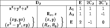
The three columns to the right are labeled according to the number and
type of operations that build up each class, 3C' ![]() refers to a
twofold axis perpendicular to the principal threefold axis. In the
next column are the labels of irreducible representation. The other
two columns list the coordinates, the quadratic forms of the
coordinates and the rotations, R
refers to a
twofold axis perpendicular to the principal threefold axis. In the
next column are the labels of irreducible representation. The other
two columns list the coordinates, the quadratic forms of the
coordinates and the rotations, R ![]() , R, R
, R, R ![]() , around the
coordinate axes.
, around the
coordinate axes.
Example: We will here give an example, regarding the water
molecule (in order to have a small system where symmetries easily can
be visualized), to show the power of group theory. In the example
symmetrical properties of the water molecule will be used to determine its
vibration modes in a very convenient way.
The water molecule belongs to the group C ![]() and have the
character table seen in table 3.3.
and have the
character table seen in table 3.3.
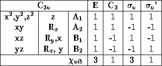
Table 3.3: The water molecules symmetry group, C ![]() .
.
![]() is here the reflection in the plane of the molecule and
is here the reflection in the plane of the molecule and
![]() ' is the reflection in the perpendicular plane bisecting the
H-O-H bond angel. The C
' is the reflection in the perpendicular plane bisecting the
H-O-H bond angel. The C ![]() axis is the z-axis that is in the plane
of the molecule and bisecting the H-O-H bond angel. The y-axis is
perpendicular to the plane of the molecule and y is perpendicular to
both x and z.
axis is the z-axis that is in the plane
of the molecule and bisecting the H-O-H bond angel. The y-axis is
perpendicular to the plane of the molecule and y is perpendicular to
both x and z.
Each atom in the molecule has 3 dimensions of freedom, an effect of
this is that the space of possible displacement is 9 dimensions. This
9-dimensional (generally called 3N-dimensional) space provides a
representation, ![]() , of the water molecules symmetry group
C
, of the water molecules symmetry group
C ![]() . It can be shown that to each vibration frequency an
irreducible representation,
. It can be shown that to each vibration frequency an
irreducible representation, ![]() , which contains
displacement modes for the atoms, can be formed. These irreducible
representations are orthogonal and together they form an
irreducible representation of C
, which contains
displacement modes for the atoms, can be formed. These irreducible
representations are orthogonal and together they form an
irreducible representation of C ![]() .
.
From the proper rotation matrix for a cartesian basis and the knowledge that only the atoms that are unmoved contribute to the character
it is seen that the character of proper rotation for the water molecule in this representation is
![]()
where N ![]() is the number of unmoved atoms. For an improper rotation
(which consists of a proper rotation followed by a reflection in the
plane perpendicular to the rotational axis) the character becomes
is the number of unmoved atoms. For an improper rotation
(which consists of a proper rotation followed by a reflection in the
plane perpendicular to the rotational axis) the character becomes
![]()
Having the characters for both proper and improper rotations of the water molecule the next step would be to remove the contributions of the three modes with zero vibration from rigid body translation and the three modes from rigid body rotation which also have a zero vibration frequency. The translation modes can be chosen to be translations along the x, y and z-axis which results in the characters
![]()
![]()
For the rigid rotations the proper rotation symmetry operation get the same character as for translation
![]()
but for improper rotations the character, which can be obtained with some vector calculus, becomes negated.
![]()
Subtracting this from the total character, ![]() , one get
the character for the remaining non-zero vibration modes,
, one get
the character for the remaining non-zero vibration modes, ![]() .
Which results in the following characters for proper and improper
rotations.
.
Which results in the following characters for proper and improper
rotations.
![]()
![]()
We can now determine the vibration characters for C ![]() s four different
symmetry elements.
s four different
symmetry elements.
¯¯¯E(proper,With this result together with a inspection of the character table for C= 0, N
= 3),

(E) = 3
C
= 1),
(improper,
) = 1
Semiconductors are a very important feature in our modern society, and the demands on performance gets higher and higher. It is therefor very important to develop new and more high performing semiconductors. In order to produce better semiconductors we have to get a deeper understanding of the atomic structure of the semiconducting material, and how doping affects the material on the microscopic level. We will in this chapter take a look at three different semiconducting materials i.e Silicon, Diamond and Silicon Carbide.
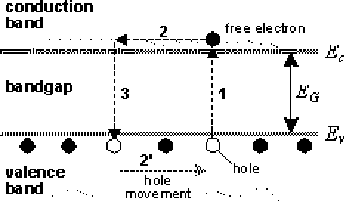
A semiconductor is a substance in which the conduction band is separated from the valence band by a band gap, E. The band gap is defined as the difference in energy between the lowest point in the conduction band and the highest point in the valence band. Bonds between atoms in semiconductors are moderately strong.
At absolute
zero temperature, all electrons are bound to their parent atoms. There
are no free electrons left that would enable electric current to flow.
Above absolute zero temperature, lattice vibrations can cause some
covalent bonds to break. A broken bond will result in a free electron,
thus enabling electric current to flow. The missing electron in a
broken bond is represented by a hole, a positive charge
carrier. Valence electrons from neighboring bonds can jump into the
place of a missing electron, contributing to electric conductivity of
the semiconductor. This process of free electron formation is called
electron-hole pair generation. As the temperature rises, the energy of lattice
vibrations increases, producing a larger amount of thermally generated
electron-hole pairs, thus increasing electrical conductivity of the
semiconductor.
Moving through the crystal, Figure:4.2, the free electron will after some time jump into another broken bond somewhere in the crystal, canceling the hole existing there at that precise moment, this process is called electron-hole recombination.
Semiconductors can be intrinsic or extrinsic, an intrinsic semiconductor is a pure semiconductor, free carriers are generated exclusively by the process of electron-hole pair generation, the concentration of free electrons equals the concentration of holes. An extrinsic semiconductor is an semiconductor with added impurities to change the electrical properties. A semiconductor in which concentration of electrons is higher than the concentration of holes is said to be an n-type semiconductor. The opposite, an semiconductor with higher concentration of holes than electrons is said to be an p-type semiconductor.
N-type semiconductors are obtained by doping the
semiconductor with an impurity, in this case called donor, with one
more valence electron than the semiconducting material. The extra
electron will be loosely bound to its parent atom and a very small amount of
energy will be sufficient to move it to the valence band.
P-type
semiconductors are obtained by adding acceptor impurities, an acceptor
impurity is an atom with one valence electron less than the
semiconducting material. Therefore, such an atom will bind an electron
that would otherwise jump from the valence band into the
conduction band, thus preventing the formation of an electron-hole pair.
Silicon is the material that today is most used as semiconducting material, it has the advantage of being easy to manufacture, and it is cheap (approx. 27% of earths crust is silicon). Today about 95% of all semiconducting devices is produced in silicon.
Pure silicon is a hard solid with a crystalline structure the same as that of the diamond form of carbon (diamond structure), to which silicon shows many chemical and physical similarities. In order to get good semiconducting properties highly purified silicon is doped with a doping material such as phosphor, which gives higher conductivity.
Natural diamonds form in the earth's mantle in regions of high temperature and high pressure, and are very rare. As new technologies have been developed for the production of artificial diamonds, the quest for diamonds has shifted more and more from the mine to the laboratory. An effect of this is that diamonds can be used in technical application at an reasonable cost. Diamond has very interesting properties for semiconducting purposes. If successful doping of diamond can be accomplished routinely, diamond devices could someday replace silicon semiconductors.
The wide-band-gap semiconductor silicon carbide have been a object of intense studies during the last few years. The reason is the unique properties of silicon carbide, these properties makes it a very interesting material for high-temperature, high-frequency and high-power applications.
The property that makes it interesting for high-energy applications is the the large electrical breakdown field strength, which is about 10 times larger than the electrical breakdown field strength for Si. SiC also has a high thermal conductivity, it can therefore operate at high temperature.
I major disadvantage with SiC is that it is very difficult to manufacture. But recent advances in crystal growth has made it possible to produce SiC of high quality. So SiC might replace Si, in applications where the use of Si is limited due to its inferior physical properties, in the nearby future.
Silicon carbide has over two hundred different crystal structures, called polytypes. All the polytypes can be build up by tetrahedrons with Si in the corners and a C placed in the center of mass of the tetrahedron. Actually it does not mater if it is Si at the corners and C in the middle or the other way around, because of symmetry.
However, the most common way to describe the structures of the different polytypes is by the use of hexagonal planes. There are three different plane configurations that can describe all the polytypes and they are here called A, B and C (see figure).
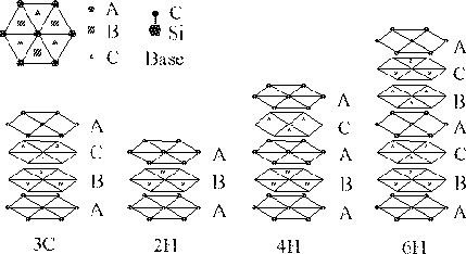
Figure 4.2: Stacking sequence of dubble layers of the three most common
SiC polytypes.
A polytype is then build up by a specific stacking sequence of the three plane types. Figure 4.2 shows one way to visualize the crystal structure with those planes.
Another way is to use the, so called, growth spiral. Starting with the tetrahedron picture, and saying that a Si atom is in the center of mass position, there will be a C atom right above this Si atom. The closest neighbor above the C atom will then consequently be one of the Si atoms occupying a site in the hexagonal plane above. From one of these new Si atoms the whole sequence can be done all over again and if the selection of the Si atom above the C atoms is done in a circular manner this will form a spiral configuration. The spiral structure representation is shown in figure 4.3.3.
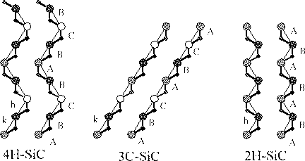
Figure 4.3: The spiral structure representation of the three most common
SiC polytupes.
If you look along the c-direction all the polytypes would look the same, since this is the direction in which all layers are stacked. But if you look at the crystals from the edge, the stacking sequence can easily be seen. 3C-Sic is the only cubic polytype of silicon carbide and it is build up by a diamond structure with Si in the fcc positions (this is called a Zinc-blend structure). It can also be described with the hexagonal layers as the stacking sequence A-B-C-A.
2H-SiC is the simplest of the hexagonal silicon carbide polytypes, it is built up by a wurtzite structure, this structure can also be described as the stacking sequence A-B-A.
The electrical properties of an semiconducting material shows how suitable the material is as an semiconductor. In silicon carbide the difference in stacking gives rise to slightly different properties, the properties of four types of SiC is shown in the table below, together with the properties of silicon and diamond.
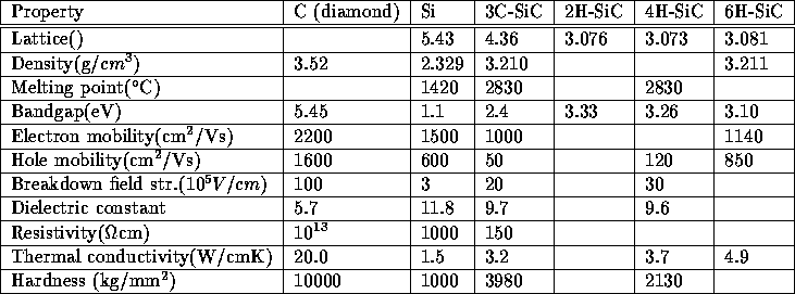
Table 4.1: Basic properties for Si, C and SiC
It is easily seen that the properties of silicon carbide and diamond are superior those of silicon. The problem is that they are very hard to dope, but intense research is being done in that area.
The purpose of this study was to examine silicon (Si) and carbon (C,
diamond) and their behavior caused by different defects, as an initial
study for silicon-carbide. The two kind of defects investigated were,
vacancies and interstitial atoms. Both of these defects are, as
mentioned before, of great interest in various aspects, but since
the vacancies appear in a quite equivalent way in pure materials we
concentrated the study to, the more complex, interstitial defect.
To do this we started to investigate hydrogen terminated
clusters with
86 atoms for both of the materials. This smaller sized cluster was
a crucial starting point which made it possible to do several
calculations, and get some general indications on the behavior of the
two materials. We then moved on to study the interstitial defect
with some alternative methods. Here we examined how two interstitial
atoms, with different start positions, reacted when they were place in
a position that conserved the symmetry of the cluster. We also relaxed
a cluster, with an interstitial atom, using the supercell technic ![]() .
Finally we continued with a study of a larger cluster consisting of 297
atoms. This last part were made with the same initial interstitial
positions as in the 86 atom cluster. We chosed the diamond structure to
be studied due to its similarities with the 3C SiC structure.
.
Finally we continued with a study of a larger cluster consisting of 297
atoms. This last part were made with the same initial interstitial
positions as in the 86 atom cluster. We chosed the diamond structure to
be studied due to its similarities with the 3C SiC structure.
The program that was used during this study was Ab initio Modeling
Program, AIMPRO
, version 5.2 that uses DFT on the basis of Hohenberg-Kohn and
Kohn-Shams discoveries in 1964 and 1965.
Calculations are based on density functional theory in either the local spin density approximation or the generalized gradient approximation. The program can model systems either in real-space (most appropriate when looking at molecular systems) or in reciprocal space using a large unit cell (most appropriate for bulk materials).
The calculations are fully self-consistent and can be either all-electron or, as is more commonly the case, using norm-conserving pseudopotentials. The wavefunction is expanded in a basis of Gaussian orbitals containing arbitrarily high angular momentum functions. Equilibrium structures are found by an efficient conjugate gradient method incorporating analytic force evaluation. Furthermore the code also evaluate dynamical properties like vibrational modes, diffusion barriers and other properties to make contact with experiments. The code is highly optimized and shows excellent scaling on parallel platforms.
The program is able to deal with two different types of boundary conditions for modeling crystalline structures. The first one, is the more common, use of supercells. This means that a part of the crystal, called a supercell, is buildt and then repeated in all directions with periodical boundary conditions. This gives a good model for pure crystalline materials, but when defects are studied this is not the optimal way of describing the structure, since even the defect is repeated periodicly. With AIMPRO it is possible to perform calculations with supercells consisting of at least 200 atoms. Because the program uses DFT with the local density approximation the program also support, unlike other Hartree-Fock based programs, so called hydrogen terminated clusters. These clusters are like the supercells, a small part taken from the crystalline structure, but instead of repeating it, hydrogen atoms are placed at the boundary to give the boundary atoms a similar environment to the one they would have if the crystal continued. With these kind of clusters AIMPRO can treat cluster sizes about 800 atoms. This gives a much more realistic model for defect crystalline structures and this is also the kind of boundary condition that was used during this study.
At first we used a, hydrogen terminated, cluster with 44 Si or C atoms and 42 H atoms, figure 5.1, to investigate the behavior of defects in this structure for the two materials.
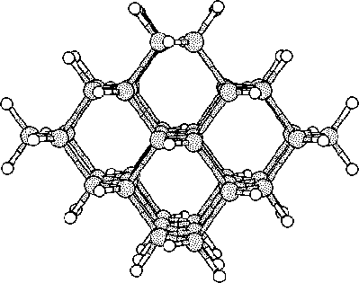
Figure 5.1: Silicon with diamond structure.
With this smaller cluster we calculated the ground state structure for a cluster with a vacancy and clusters with interstitial atoms. The interstitial atoms were of the same kind as the atoms which builds up the cluster. We used three different initial positions of the interstitial atoms to conclude where an arbitrary interstitial atom are most likely to end up.
The result from the carbon vacancy calculation showed that with the lack of an atom the relaxed structure is the same as the initial one, but the neighbors are a bit pushed away from the empty atom site. This due to the fairly strong bonds of carbon. The interstitial atoms, on the other hand, did not give that predicted results. Three different initial positions of the interstitial atoms were used, figure 5.2.
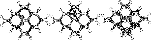
Figure 5.2: The three different start positions of the interstitial
atoms, in the carbon cluster. The red ring marks the interstitial atom.
The left of figure 5.2 shows a interstitial atom which are place approximately at the same site as another atom. In the middle an interstitial atom with equal distance to all equivalent neighbors, i.e. no preferred moving direction, can be seen. The right part shows a interstitial placed directly on a bond, with equal distance to the two atoms. After the calculations the clusters had relaxed to the following structures, figure 5.3.
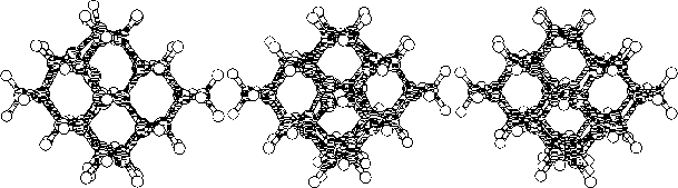
Figure 5.3: The three relaxed interstitial clusters.
The conclusion of these results were that the interstitial atom strive for a position at a bond. It seems like the final position can differ a bit, depending of the atoms start position, but one should keep in mind that the cluster is very small.
The same strategy was used in the case with Si. The relaxed vacancy showed that the neighboring atoms were pulled together, towards the atom site with an atom missing, figure 5.4.
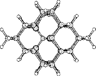
Figure 5.4: Relaxed silicon cluster with vacancy. It can be seen that the
marked atoms have moved closer together around the free atom site.
This is because of the weaker bonds and Silicons larger core. For the study of interstitial atoms the same three positions as in the carbon analysis were, used figure 5.5.
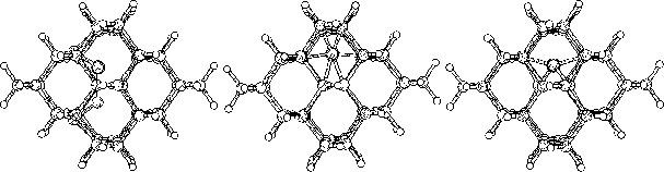
Figure 5.5: The three different start positions of the interstitial
atoms, in the silicon cluster
The only difference compared to the carbon clusters was that the interstitial atom that was placed at the middle of a bond now was placed above two atoms, but with a smaller distance to them than the other surrounding atoms. This was done because the position right in the middle of a bond would give a rather extreme situation due to the properties of silicon. After the relaxation we got the following results, figure 5.6.
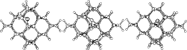
Figure 5.6: The three relaxed interstitial clusters.
The silicon gave a similar result as carbon. The difference was that it had a more independent placement of the interstitials. All three relaxed clusters had a more or less equivalent position of there interstitial atoms, and there ground state energies were very similar. Because of the weaker bonds in silicon it is also seen that the interstitial atoms are located at larger distances from the bonds than in carbon.
We performed two different calculations on interstitial atom defects where the interstitial atom were placed in a position where the total symmetry were conserved, see figure 5.7. The cluster used consisted of 72 bulk atoms (Si or C) and 60 hydrogen atoms.
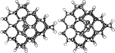
Figure 5.7: The two different start positions of the interstitial atoms
in the 132-atom cluster.
The purpose of this was to see if the symmetry affected the final position of the interstitial atom. Because of these clusters larger size they were calculated in a more careful manner so that a comparison of energy would be possible. We also made a calculation on an interstitial atom in a supercell, as a complement to our hydrogen terminated calculations.
After relaxation we got the following structures from the diamond cluster.
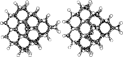
Figure 5.8: The two different end positions of the interstitial
atoms in the 132-atom carbon cluster
Seen in figure 5.8, the left cluster roughly mainteined its initial structure. The right one changed its structure during relaxation and as the figure shows an atom is drawn towards the middle of a bond. The result of the calculations also showed that the left interstitial configuration had the lower ground state energy (in the order of 1.9 eV).
The result from the silicon relaxation differed a bit from the result of carbon.
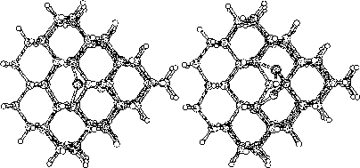
Figure 5.9: The two different end positions of the interstitial
atoms in the 132-atom silicon cluster
The left structure became a bit perturbed, but had again a quite similar structure, as in the case with carbon. Unlike the result from the second carbon cluster the silicon maintained its initial structure. The two structures had almost the same ground state energy (differs less than 0.4 eV).
In the supercell, consisting of 64 silicon atoms, we placed the interstitial atom so that it shared site with one of the original atoms, see right part of figure 5.10. This is similar to the first interstitial configuration for the 86-atom cluster.
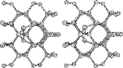
Figure 5.10: The silicon supercell
The right part of figure 5.10 shows the relaxed structure. This structure is rather similar to the initial structure, but the atom par consisting of the interstitial and its sharing atom has moved to a more centered position relative the hexagonal pattern.
No further conclusions were drawn at this stage, instead we continued and saved this to compare with the results from the larger cluster.
The next step was to use the bigger cluster to create a more physically correct environment for the interstitial atom and compare the result to our previous results. A 297-atom cluster was used and in this cluster interstitial atoms were made with the same initial positions as in the 86-cluster. The initial, undefected, cluster consisted of 181 Si or C atoms and 116 H atoms. Figure 5.11 shows the undisturbed 297-atom cluster.
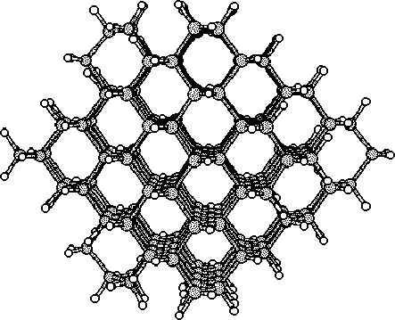
Figure 5.11: The undefected 297-atom cluster.
The size of the larger cluster made it relevant to compare the energy of the different final structures and . The relaxed interstitial clusters, figure 5.12, were carefully calculated in order make this comparison possible.
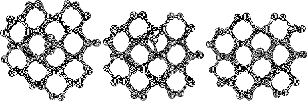
Figure 5.12: The three relaxed diamond clusters.
The three final structures had very similar ground state energies. They differed about 0.5 eV each. The structure with the lowest ground state energy was the interstitial atom with a initial position with no preferred moving direction, showed in the middle part of figure 5.12. The structure with second lowest energy was structure where the start position of the interstitial was on a bond, right in figure 5.12. The structure with the highest energy was the one where the initial interstitial atom was sharing a site with another atom, left in figure 5.12.
Figure 5.13 shows the final structures of the large silicon clusters.
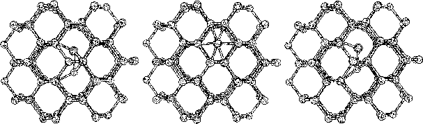
Figure 5.13: The three relaxed silicon clusters.
Even here the ground state energies were similar, but a difference was noticed. The structure with lowest energy was the one where the interstitial atom started with no preferred direction to move in. The other two were practically equal (differed less than 0.05 eV) and they differed about 0.5 eV from the lowest structure.
This study showed that the ground state structure of silicon and carbon differs when a defect, such as an interstitial atom or a vacancy, is present.
When a vacancy is appears in carbon the surrounding atoms are pulled away from the empty site. The reason to this behavior is most likely the strong bonds of carbon. The vacancy in silicon acts in the opposite way. The surrounding atoms pushed towards the vacancy, and this due to there weaker bonds and larger core.
The interstitial atoms are a more complex defect, and the results were therefor harder to interpret. Even though some different structures apeared a over all characteristic behavior could be noticed. From the results of the large carbon cluster it is observed that, in the two structures with the lowest energies, the interstitial atom has been pulled towards a bond in the cluster. This behavior can also be seen in the 86-atom clusters, as well as in one of the cluster with 132 atoms.
In silicon we also detected a characteristic behavior of the interstitial atoms. The result from the calculations of the 298-atom cluster showed that both the interstitial atom which started in the same site as another atom and the interstitial who started at a bond relaxed to very similar structures. The final structure of those two interstitials was a structure where each interstitial shared a site with an other atom. This relaxed structure could also be seen in the result of the supercell and in one of the 132-atom clusters. The 86-atom cluster did not show any signs of this behavior but the reason for this could be that the cluster was to small to create a physically correct environment.
How the symmetry affected the calculations on the 132-atom cluster is hard to tell, but if an interstitial atom is placed not to close to a local minimum the interstitial atom seams relax into a correct position.
In this report we have made structural calculations on silicon and carbon with Density Functional Theory. We have studied the effects of introduced interstitials and vacancies on the structure. These kinds of defects are not yet well understood and accurate experimental data lack.
We have found that DFT is a very powerful tool for making these kinds of calculations and that realistic results can be obtained with a limited effort, as well computationally as human. It is rather surprising that such a simple scheme as that of Kohn-Sham can give so exact results. In short, the idea of the method is use the electron density as the fundamental variable instead of the wave-function, as would have been the case otherwise. This reduces the number of variables drastically. For the ground state of the system, this representation is exact. Excited states are not possible to calculate with any good accuracy, but there is a lot of information to extract from the ground state in itself. For example Finally, during tihs project we have gained understanding in the structural calculations on multi-particle systems such as real semiconductors. We have penetrated the theory that forms the foundations of the Density Functional Theory and we have made practical calculations to see how well the theory fits with reality. The work has brought us a broad experience, as well of the diverse subjects, as of the procedures that are required when a larger project with several people involved shall be executed. A procedure that will often present itself in the future.
There are only two ways to live your life. One is as though nothing is a miracle. The other is as though everything is a miracle.
- Albert Einstein
A functional F[y] is a mapping that takes an element y from a given set Y and produces a real (or complex) number c.
![]()
In this work we deal mainly with Y as a Hilbert space, H, and y as a function.
In the theory of functionals y could also be e.g. a matrix or a sequence. Here are some examples
where ![]() :
:
![]()
![]()
![]()
The element in DFT is the electron density ![]() and the space is the set of functions with
and the space is the set of functions with
![]()
This means that the particle density cannot be negative, that the integral over all space must
equal the total number of electrons and that the electron density doesn't vary unphysically.
This is a Hilbert space with the inner product ![]() .
.
The functional derivative ![]() is defined by:
is defined by:
![]()
where F is the functional of ![]() .
For example the Tomas Fermi energy
.
For example the Tomas Fermi energy
![]()
has the derivative:
Caution: If the functional contains for example a differential operator this does not
commute with ![]() . For example:
. For example:
This can be expressed generally. Let
![]()
where ![]() =
= ![]() is the partial derivative.
Then, if
is the partial derivative.
Then, if ![]() vanishes on the boundary of
vanishes on the boundary of ![]() ,
,
![]()
according to Gelfand and Fomin 1963 [1], p. 42. This formula can be used to find (A.5) directly.
In the same way as in ordinary calculus an extrema of a functional is obtained when
![]()
This means that if we make a small variation of the function ![]() this won't change
the value of the functional.
With a constraint
this won't change
the value of the functional.
With a constraint
![]()
on the functional ![]() we can employ the method of Lagrangian multipliers, i.e.
to solve the auxiliary Euler-Lagrange equation:
we can employ the method of Lagrangian multipliers, i.e.
to solve the auxiliary Euler-Lagrange equation:
![]()
without the constraint and then impose it to find the multiplier ![]() .
.
For most of our applications we will be interested in the constraint:
![]()
which gives the Euler-Lagrange equation:
![]()
Even if this condition is satisfied, we are only guaranteed a local maximum or minimum. Fortunately, the physical situation often excludes the possibility of a maximum, and as for locality physical arguments only can tell us whether the minimum is local or global.
This document was generated using the LaTeX2HTML translator Version 96.1 (Feb 5, 1996) Copyright © 1993, 1994, 1995, 1996, Nikos Drakos, Computer Based Learning Unit, University of Leeds.
The command line arguments were:
latex2html -split 0 -show_section_numbers Struct.tex.
The translation was initiated by Erik Elfgren on Tue Mar 28 09:54:28 MET DST 2000
45#45
where 46#46 forms an 47#47 matrix and N is the number of fermions in the system. This reduces to
48#48
in the simple case of two electrons.
 .
.
126#126